Paradigm's latest research: The financial alchemy of Uniswap

The original authors are researchers Dave White, Martin Tassy, Charlie Noyes, and Dan Robinson from the investment firm Paradigm, who are also seed investors in Uniswap.

Under ruthless arbitrage, Uniswap LPs have become wealthy (source).

1. Problem
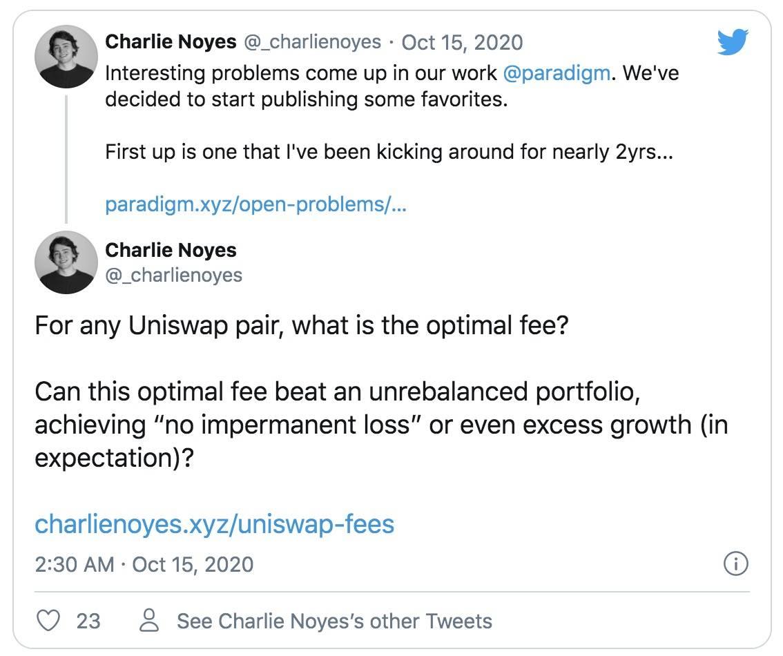
On October 14, Charlie Noyes posted a question on Twitter that he and Dan Robinson had been debating:

"What is the optimal fee for any Uniswap asset pair? Can this optimal fee outperform an unbalanced portfolio, eliminating impermanent loss and even achieving excess growth?"

1.1 Background

Automated Market Makers (AMMs) are a type of decentralized exchange that allows customers to trade between on-chain assets like USDC and ETH. Uniswap is the most popular AMM on Ethereum, and like most asset management systems, Uniswap facilitates trading between specific asset pairs by holding reserves of two assets. It determines the trading price between them based on the size of its reserves, keeping prices aligned with the broader market.

Anyone willing to join a particular asset pool is referred to as a liquidity provider, or LP for short. These individuals contribute assets to both reserve assets and take on some trading risk in exchange for a portion of the transaction fee returns.

1.2 Setting the Problem

The asset pool provides liquidity between stablecoins and risk assets with price fluctuations, and we make a particularly harsh assumption that all trades entering the pool are informed (arbitrage trades only occur when there is a deviation between the AMM price and the normal trading price).

In other words, the entire pool experiences losses after each trade.

1.3 Traditional Thinking

At first glance, becoming a Uniswap LP in this scenario seems like a costly mistake.

Market makers require the buy price to be lower than the sell price, so when asset prices remain stable, they profit directly, achieving a roughly balanced buy and sell volume. These trades are often referred to as "uninformed" trades because they are unrelated to short-term price movements.

On the other hand, market makers incur losses when they buy assets before a price drop or sell before a price increase. Therefore, one of the market makers' biggest fears is arbitrageurs, who only trade when prices change, leaving market makers behind. Each trade executed by arbitrageurs is pure profit for them, while it represents pure loss for market makers.

Since there are no uninformed trades in our Uniswap problem setup (in fact, we assume every trade is an arbitrage trade), LPs will clearly experience significant losses.

1.4 Challenge

However, Dan and Charlie believe the story does not end there.

They suspect that for certain potential price dynamics, becoming a Uniswap LP still makes sense.

They posed this question to the legendary figure in mathematical finance, Steven Shreve, and then published it on Twitter. Martin Tassy and I independently proposed partial solutions and then collaborated to extend the complete solution to general cases.

In the following weeks, the four of us spent some time discussing results via Telegram, looking for errors, and building our intuition, which formed the basis of this article.

2. Solution

If the volatility of an asset is sufficiently high relative to its average return, then over time, LPs on Uniswap will outperform HODLers, even in a scenario where all trades are arbitrage trades.

This is due to a phenomenon known as "volatility harvesting": under certain conditions, periodically rebalancing the two assets can lead to performance that exceeds any static portfolio. In this context, "rebalancing" refers to trading to return the proportion of total asset value held in each asset to a fixed allocation, such as 50/50.

Thus, when LPs are arbitraged, they essentially pay a fee to the market to rebalance their portfolio. In this specific mathematical environment, when such rebalancing is beneficial, you want to do it as much as possible. This means liquidity providers should set their fees as low as possible without being zero.

This is good news for Uniswap, as it means that even in a scenario dominated by arbitrage trading, low fees can still be enjoyed, keeping Uniswap competitive as on-chain orders increase and begin to offer smaller spreads.

That said, it is worth repeating that these results apply to a very specific formalized mathematical setting, where the assumptions involved are very similar to those in the Black-Scholes option pricing model. For mathematical convenience, we also assume a fee structure different from that used in Uniswap production.

2.1 Benchmarking

We evaluate different strategies by comparing their asymptotic wealth growth rates, which measure how quickly they compound (or lose) value over the long term.

This quantity is important because optimizing it over time performs better than executing a strategy that is nearly uncertain.

We compare all strategies against an "unbalanced portfolio," which holds half its value in stablecoins and half in risk assets, and never changes thereafter. This is also the community standard for measuring the so-called "impermanent loss" in AMMs.

Regardless of what happens, the unbalanced portfolio always holds the same amount of stablecoins, meaning that in the worst-case scenario, when the risk asset loses all its value, the unbalanced portfolio will consist almost entirely of stablecoins, leading to a long-term growth rate of zero.

On the other hand, if the risk asset experiences exponential growth, it will quickly dominate the unbalanced portfolio, and its growth rate will match that of the risk asset.

It is noteworthy that two portfolios can share the same asymptotic wealth growth rate while performing very differently in the near term. For example, if the growth rate of the risk asset is zero, then the value of the zero-fee Uniswap shares will always be less than that of the unbalanced portfolio, but since both are expected to neither compound growth nor loss over time, their wealth growth rates will both be zero.

2.2 Volatility Drag

Volatility drag during a 50% loss/75% gain process (source).
To understand these results, it is essential to grasp the concept of volatility drag. Suppose our risk asset has a price that either drops 50% or rises 75% each year, with both outcomes being equally probable.

In any given year, if we invest $100 in that asset, our expected value is (50 + 175) / 2 = $112.5. If we simply buy and hold, our portfolio's expected value would increase by 12.5% each year, which seems like a good deal.

Unfortunately, in the real world, our profits do not materialize. If we buy and hold this security, we ultimately lose everything.

This is because, over time, the compounding of wealth leads to catastrophic losses.

If we lose 50% in one year and then gain 75% the next, we end up with only 87.5% of our initial investment (i.e., 50% * 175%).

Over time, the law of large numbers guarantees our returns will be -15% each year, and we will inevitably go bankrupt.

2.3 Wait, What Happened?

If you have been trained to analyze gambling from the perspective of expected value, then the previous section may seem very strange, or even completely incorrect.

In fact, just over a week ago, we had a complete, closed-form mathematical solution to this problem, and prior to that, I had no idea what it intuitively meant.

The root of the issue is that expected value is a theoretical quantity that measures what would happen if we replicated a given game across countless parallel universes simultaneously.

But reality is not like that; we only have one chance at each game, and the effects of the games we play are not instantaneous but compound over time.

We can look at it from another angle to help reconcile the mathematics. As we repeatedly engage in the (-50% / +75%) game, reinvesting funds each time, only a very few paths are correct, leading to astronomical returns.

Over time, the proportion of these paths among all possible paths shrinks, and the chance of actually seeing one of those paths realized also approaches zero.

2.4 The Value of Rebalancing

In the face of volatility drag, even when expected values are positive, it is wise to set aside some funds. This way, when things go wrong, your losses will be mitigated, increasing your compounded wealth in the long run.

In trading, all of this leads to some fairly familiar concepts. When prices rise, sometimes it makes sense to close part of a position to lock in profits in case prices drop again. When prices fall, sometimes it makes sense to buy the dip to gain expected future returns at a favorable price.

In some cases, like this one, the best strategy is to continuously rebalance your portfolio so that you always have a fixed proportion of wealth invested in each position, say, half in stablecoins and half in risk assets. This is not always the optimal balance; generally, you want more risk assets in your portfolio, the higher their return relative to their volatility, but we will postpone further exploration of this to future work.

The benefits of rebalancing for long-term wealth growth can be enormous, potentially making the difference between exponential wealth growth and bankruptcy. Even in the context we set up, each rebalancing trade has an unfavorable price and incurs an instantaneous loss, which is also a fact.

2.5 Resources

You may find yourself dissatisfied with these explanations and want to learn more.

You can start by reviewing the Kelly Criterion, which is a theoretically optimal betting strategy based on these principles. @wpoundstone's book, The Fortune Formula, is a well-regarded and easy-to-read account of the history and implications of the Kelly Criterion.

On the other hand, for an in-depth study of the mathematics of wealth growth, I highly recommend @olebpeters's lecture notes on ergodic economics here or his article published in Nature here.

If you choose to research this on your own, be cautious; it is a little-known field, and in my own research process, I found many sources with errors that set back my understanding by hours or days.

In particular, if you see someone invoking mean reversion or logarithmic utility functions, I suggest you do not linger and move on. The key results in this field do not require the assumption of any specific return distribution or utility function.

2.6 Fee Alchemy

In this setup, when is it beneficial to become an LP, and how often should LPs rebalance to facilitate rebalancing at minimal cost?

(Fee levels should be as low as possible but not zero, to trigger rebalancing through increasingly minor price changes. Dan Robinson refers to this as "picking up pennies in a quantum foam.")

However, when fees are completely zero, all the benefits of rebalancing disappear, and in most cases, LPs are worse off than if they simply held an unbalanced portfolio.

Understanding this seemingly counterintuitive phenomenon helps reveal the rest of the problem.

Uniswap uses a "constant product" invariant, meaning that without fees, each trade must keep the product of the reserve balances constant. We express this as , although readers familiar with Uniswap may be more accustomed to writing it as x*y = k.

However, it turns out that to achieve rebalancing, the number C of this product must increase to provide us with excess wealth growth.

Why is C so important? We say that is the geometric mean of our reserve balances Ra and Rb. Like the arithmetic mean, the geometric mean increases with the amount of reserves. However, unlike the arithmetic mean, the geometric mean shrinks as the reserves become unbalanced, even if their arithmetic mean remains constant.

With no fees, C remains constant, so trades always lead to either larger reserves or more balanced reserves. Both cannot exist simultaneously, so there is no incentive for wealth growth.

However, in the real-world Uniswap, or in our set environment, non-zero fees ensure that C increases with each trade. Over time, this means that reserves not only grow but also remain balanced, providing the benefits discussed above.

To understand the precise mathematics of how this is calculated, refer to section 3.1 of the proof paper by Martin and me.

3. Mathematics

Having said all this, we can now accurately answer the question posed in Charlie's original statement.

To reiterate, they are concerned with the wealth growth rate G of Uniswap-style AMMs, where the percentage fee rate affects the market between stablecoins and volatile assets (which follow geometric Brownian motion volatility, with parameters drift and volatility).

3.1 LP Wealth Growth Rate

3.2 Optimal Fees and Excess Returns

An LP holding half stablecoins and half risk assets will outperform simply holding assets if and only if:

In this case, LPs should set their fees as low as possible but not zero, and they will achieve a wealth growth rate that gradually approaches .

3.3 Explanation

Since geometric Brownian motion simulates compound growth, it is also subject to volatility drag, mathematically represented as , with a wealth growth rate of:

This means that within the range of , becoming a Uniswap LP is more meaningful than the growth rate of a HODL of .

This gives us a perspective on the observation: rebalancing allows us to partially offset the volatility drag of the underlying assets. If there were no volatility drag, and the average return were zero or negative, then the amount of rebalancing would be of no use. Although the rebalanced portfolio would still perform better than simply holding the assets themselves, we would be better off just holding stablecoins.

On the other hand, if the average return without volatility drag is positive:

1. If the volatility drag causes asset losses exceeding 200% of its average logarithmic return, then rebalancing on Uniswap will not eliminate enough drag, and you would be better off holding stablecoins.

2. If the volatility drag causes asset losses below 66% of its average logarithmic return, then rebalancing on Uniswap is not worthwhile, and you would be better off simply holding the asset.

3. Within this range, becoming a Uniswap LP will ultimately make you wealthy, in fact, more so than holding any unbalanced portfolio composed of stablecoins and volatile assets. This includes some assets that will ultimately become worthless and some that will exhibit parabolic growth.

3.4 Proof

You can find the complete proof in the preprint paper here. It works by establishing a dynamical model for discrete random walks and then taking limiting behavior as the step size approaches zero.

You can also check my original proof for the zero-logarithmic-drift case and simulate some problems here.

3.5 How much trust should we place in these findings?

In my personal view, they are quite credible.

We have two independent proof methods that yield the same results when their domains overlap. We also have some simulations that validate our predictions:

Simulated vs. predicted wealth growth rates (source).
Nevertheless, this remains a very confusing field, and my understanding of it has changed many times over the past few weeks. If you do find errors, please feel free to reach out to us.

4. Future Work

While we hope you agree that these findings are theoretically interesting (or perhaps maddening), there is still a great deal of work to be done to determine their relevance to the real world.

For example, many of our assumptions can be modified or extended:

1. How can we translate these results into multi-asset cases, or when can LPs choose ratios other than 50/50 like Balancer for rebalancing?

2. What happens when we no longer allow unlimited trades per unit of time?

3. What if we introduce trading costs that can even vary to reflect priority gas auction dynamics?
   There are also some empirical questions:

4. Can we estimate these parameters for securities trading in today's markets?

5. How many actively traded tokens could benefit from the rebalancing strategy we described?

6. Can we determine what proportion of realized Uniswap LP returns in reality is due to volatility harvesting?
   Finally, perhaps most interestingly, how can we apply the knowledge gained here to improve existing protocols, create a new protocol, or develop the DeFi ecosystem as a whole?
   5. Let’s Discuss Together

Any questions? Thoughts? Potential applications?

We want to hear your voice.

@charlienoyes ● @danrobinson ● @Dave_White ● @MartinTassy

Thanks to Vitalik Buterin, Matt Huang, Georgios Konstantopoulos, and Alex Evans for their feedback on this article.