LUCIDA & FALCON: Building a Strong Crypto Asset Portfolio with Multi-Factor Strategies

Author: LUCIDA & FALCON

Preface

Continuing from our last article, we have published the first part of the series "Building a Strong Cryptocurrency Asset Portfolio with Multi-Factor Strategies" --- Theoretical Foundation. This is the second part --- Data Preprocessing.

Before calculating factor data and testing the effectiveness of individual factors, relevant data needs to be processed. Specific data preprocessing involves handling duplicates, outliers/missing values/extreme values, normalization, and data frequency.

1. Duplicates

Data-related Definitions:

• Key: Represents a unique index. eg. For a dataset containing all tokens for all dates, the key is "tokenid/contractaddress - date".
• Value: The object indexed by the key is referred to as the "value".

To diagnose duplicates, one must first understand what the data "should" look like. Typically, the forms of data are:

1. Time Series Data. The key is "time". eg. Price data for a single token over 5 years.
2. Cross Section Data. The key is "individual". eg. Price data for all tokens in the crypto market on 2023.11.01.
3. Panel Data. The key is a combination of "individual-time". eg. Price data for all tokens from 2019.01.01 to 2023.11.01 over four years.

Principle: Once the index (key) of the data is determined, one can know at what level there should be no duplicates.

Checking Methods:

1. pd.DataFrame.duplicated(subset=[key1, key2, ...])

   Check the number of duplicates: pd.DataFrame.duplicated(subset=[key1, key2, ...]).sum()

   Sample to see duplicate entries: df[df.duplicated(subset=[...])].sample() After finding the sample, use df.loc to select all duplicate samples corresponding to that index.

2. pd.merge(df1, df2, on=[key1, key2, ...], indicator=True, validate='1:1')

   In the horizontal merge function, adding the indicator parameter will generate a _merge field. Using df['_merge'].value_counts() can check the number of samples from different sources after merging.

   Adding the validate parameter can check whether the indexes in the merged dataset are as expected (1 to 1, 1 to many, or many to many, where the last case actually does not require validation). If it does not match expectations, the merge process will raise an error and stop execution.

2. Outliers/Missing Values/Extreme Values

Common Causes of Outliers:

1. Extreme Cases. For example, a token price of $0.000001 or a token with a market cap of only $500,000 can yield dozens of times returns with just a slight fluctuation.

2. Data Characteristics. For instance, if token price data is downloaded starting from January 1, 2020, it is naturally impossible to calculate the return rate for January 1, 2020, because there is no closing price from the previous day.

3. Data Errors. Data providers inevitably make mistakes, such as recording a price of 12 yuan per token as 1.2 yuan per token.

Principles for Handling Outliers and Missing Values:

1. Deletion. For outliers that cannot be reasonably corrected or fixed, deletion may be considered.

2. Replacement. Typically used for handling extreme values, such as Winsorizing or taking logarithms (less common).

3. Filling. For missing values, reasonable filling methods can be considered, common methods include mean (or moving average), interpolation, filling with 0 df.fillna(0), forward filling df.fillna('ffill')/backward filling df.fillna('bfill'), etc. It is essential to consider whether the assumptions underlying the filling are valid.

   Machine learning should be cautious with backward filling due to the risk of look-ahead bias.

Methods for Handling Extreme Values:

1. Percentile Method.

By ordering the data from smallest to largest, data exceeding the minimum and maximum percentiles are replaced with critical values. This method is relatively rough for datasets with rich historical data and may cause a certain percentage of loss by forcibly deleting a fixed proportion of data.

2. 3σ / Three Standard Deviations Method

The standard deviation σ factor reflects the dispersion of factor data distribution, i.e., volatility. Using the range μ±3×σ to identify and replace outliers in the dataset, approximately 99.73% of the data falls within this range. The prerequisite for this method: Factor data must follow a normal distribution, i.e., X∼N(μ,σ²).

Where, μ=∑ⁿᵢ₌₁⋅ Xi / N, σ²=∑ⁿᵢ₌₁=(xi -μ)²/ n, the reasonable range for factor values is [μ−3×σ, μ+3×σ].

Adjust all factors within the data range as follows:

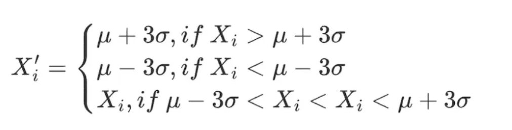The drawback of this method is that commonly used data in the quantitative field, such as stock prices and token prices, often exhibit heavy-tailed distributions and do not conform to the assumption of normal distribution. In such cases, using the 3σ method may incorrectly identify a large amount of data as outliers.

3. Median Absolute Deviation Method (MAD)

This method is based on the median and absolute deviation, making the processed data less sensitive to extreme or outlier values. It is more robust than methods based on mean and standard deviation.

The median absolute deviation is defined as MAD = median(∑ⁿᵢ₌₁( Xi - X median )).

The reasonable range for factor values is [X median - n × MAD, X median + n × MAD]. Adjust all factors within the data range as follows:

# Handling Extreme Values in Factor Data
class Extreme(object):
    def __init__(s, ini_data):
        s.ini_data = ini_data

    def three_sigma(s, n=3):
        mean = s.ini_data.mean()
        std = s.ini_data.std()
        low = mean - n * std
        high = mean + n * std
        return np.clip(s.ini_data, low, high)

    def mad(s, n=3):
        median = s.ini_data.median()
        mad_median = abs(s.ini_data - median).median()
        high = median + n * mad_median
        low = median - n * mad_median
        return np.clip(s.ini_data, low, high)

    def quantile(s, l=0.025, h=0.975):
        low = s.ini_data.quantile(l)
        high = s.ini_data.quantile(h)
        return np.clip(s.ini_data, low, high)

3. Normalization

1. Z-score Normalization

• Prerequisite: X ~ N(μ, σ)
• Due to the use of standard deviation, this method is sensitive to outliers in the data.

x'ᵢ=(x−μ)/σ=(X−mean(X))/std(X)

2. Min-Max Scaling

Transforms each factor data into values within the (0,1) range for comparison of data of different scales or ranges, but it does not change the internal distribution of the data nor does it make the sum equal to 1.

• Sensitive to outliers due to consideration of extreme values.
• Uniform scale, facilitating comparison of data across different dimensions.

x'ᵢ=(xᵢ−min(x))/(max(x)−min(x))

3. Rank Scaling

Transforms data features into their ranks and converts these ranks into scores between 0 and 1, typically their percentiles in the dataset.

• Since ranks are not affected by outliers, this method is insensitive to outliers.

• Does not maintain the absolute distances between points in the data but converts them into relative ranks.

NormRankᵢ=(Rankₓᵢ−min(Rankₓ))/(max(Rankₓ)−min(Rankₓ))=Rankₓᵢ/N

Where, min(Rankₓ)=0, N is the total number of data points in the range.

# Normalizing Factor Data
class Scale(object):
    def __init__(s, ini_data, date):
        s.ini_data = ini_data
        s.date = date

    def zscore(s):
        mean = s.ini_data.mean()
        std = s.ini_data.std()
        return s.ini_data.sub(mean).div(std)

    def maxmin(s):
        min = s.ini_data.min()
        max = s.ini_data.max()
        return s.ini_data.sub(min).div(max - min)

    def normRank(s):
        # Rank the specified column, method='min' means that identical values will have the same rank, rather than an average rank.
        ranks = s.ini_data.rank(method='min') 
        return ranks.div(ranks.max())

4. Data Frequency

Sometimes the data obtained does not match the frequency needed for our analysis. For example, if the analysis level is monthly and the original data frequency is daily, "downsampling" is required, i.e., aggregating the data to a monthly frequency.

Downsampling

Refers to aggregating the data in a set into a single row of data, such as aggregating daily data into monthly data. At this point, the characteristics of each aggregated metric need to be considered, with common operations including:

• First value/Last value
• Mean/Median
• Standard deviation

Upsampling

Refers to splitting a single row of data into multiple rows, such as using annual data for monthly analysis. In this case, simple repetition is generally sufficient, and sometimes annual data needs to be proportionally allocated to each month.

About LUCIDA & FALCON

Lucida (https://www.lucida.fund/) is an industry-leading quantitative hedge fund that entered the crypto market in April 2018, primarily trading strategies such as CTA/statistical arbitrage/option volatility arbitrage, and currently manages $30 million.

Falcon (https://falcon.lucida.fund) is a next-generation Web3 investment infrastructure based on multi-factor models, helping users "select," "buy," "manage," and "sell" cryptocurrency assets. Falcon was incubated by Lucida in June 2022.

For more content, visit https://linktr.ee/lucida_and_falcon