Build a Strong Cryptocurrency Asset Portfolio with Multi-Factor Strategies #Macro Factor Analysis: Factor Synthesis#

^Author: LUCIDA \& FALCON^

Continuing from the last time, in the series of articles on "Building a Strong Cryptocurrency Asset Portfolio with Multi-Factor Models," we have published three articles: “Theoretical Foundation”, “Data Preprocessing”, and “Factor Effectiveness Testing”.

The first three articles explain the theory of multi-factor strategies and the steps for single-factor testing.

1. Reason for Factor Correlation Testing: Multicollinearity

We have filtered out a batch of effective factors through the single-factor testing section, but the above factors cannot be directly stored. Factors themselves can be classified into broad categories based on their specific economic meanings, and there is a strong correlation among similar types of factors. If we directly store them without correlation screening, when performing multiple linear regression to obtain expected returns based on different factors, multicollinearity issues will arise. In econometrics, multicollinearity refers to the existence of "perfect" or exact linear relationships among some or all explanatory variables in a regression model (high correlation among variables).

Therefore, after filtering effective factors, we first need to conduct T-tests on the correlation of factors based on broad categories. For factors with high correlation, we either discard those with lower significance or perform factor synthesis.

The mathematical explanation of multicollinearity is as follows:

Consequences of multicollinearity:

1. Parameter estimates do not exist under perfect collinearity.

2. Under approximate collinearity, OLS estimates are inefficient.

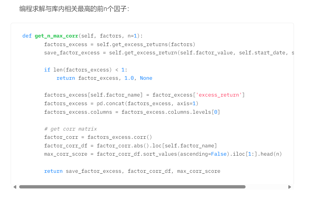
2. Step 1: Correlation Testing of Similar Factors

Test the correlation between newly derived factors and stored factors. Generally, there are two types of data for correlation testing:

1. Calculate correlation based on the factor values of all tokens during the backtesting period.

2. Calculate correlation based on the excess return values of all tokens during the backtesting period.

3. Step 2: Factor Selection and Synthesis

For collections of factors with high correlation, two approaches can be taken:

(1) Factor Selection

Select the most effective factors based on their ICIR values, returns, turnover rates, and Sharpe ratios, retaining them while deleting others.

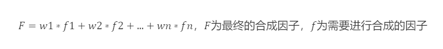
(2) Factor Synthesis

Synthesize the factors in the factor collection, retaining as much effective information as possible in the cross-section.

Assume there are currently three factor matrices to be processed:

synthesis = pd.concat([a,b,c],axis = 1) 
synthesis
a    b   c
BTC.BN    0.184865    -0.013253   -0.001557
ETH.BN    0.185691    0.022708    0.031793
BNB.BN    0.242072    -0.180952   -0.067430
LTC.BN    0.275923    -0.125712   -0.049596
AAVE.BN    0.204443    -0.000819   -0.006550
...    ... ... ...
SOC.BN    0.231638    -0.095946   -0.049495
AVAX.BN    0.204714    -0.079707   -0.041806
DAO.BN    0.194990    0.022095    -0.011764
ETC.BN    0.184236    -0.021909   -0.013325
TRX.BN    0.175118    -0.055077   -0.039513

2.1 Equal Weighting

Each factor has equal weight (w=1/number of factors), and the composite factor is the average of the sum of each factor's values.

For example, for momentum factors, the one-month return, two-month return, three-month return, six-month return, and twelve-month return, each of these six factors contributes 1/6 of the weight to synthesize a new momentum factor load, which is then standardized again.

`synthesis1 = synthesis.mean(axis=1) # Calculate mean by row

`

2.2 Historical IC Weighting, Historical ICIR, Historical Return Weighting

Weight the factors using the IC values (ICIR values, historical return values) from the backtesting period. There have been many periods in the past, each with an IC value, so their average is used as the weight of the factors. Typically, the mean of the IC during the backtesting period (arithmetic mean) is used as the weight.

# Weight normalization (the factor weighting methods mentioned later also generally require weight normalization)
w_IC = ic.mean() / ic.mean().sum()
w_ICIR = icir.mean() / icir.mean().sum()
w_Ret = Return.mean() / Return.mean().sum()
synthesis2 = (synthesis * w_IC).sum(axis=1)
synthesis2 = (synthesis * w_ICIR).sum(axis=1)
synthesis2 = (synthesis * w_Ret).sum(axis=1)

2.3 Historical IC Half-Life Weighting, Historical ICIR Half-Life Weighting

Both 2.1 and 2.2 calculate the arithmetic mean, assuming that each IC and ICIR during the backtesting period has the same effect on the factors.

However, in reality, each period during the backtesting period does not have the same level of influence on the current period, and there is a time decay. The closer the period is to the current period, the greater the influence; the farther away, the smaller the influence. Based on this principle, before calculating IC weights, we first define a half-life weight, where the weight value is larger the closer it is to the current period and smaller the farther away.

Mathematical derivation of half-life weight:

2.4 Maximizing ICIR Weighting

Calculate the optimal factor weight w that maximizes ICIR by solving the equation.

Estimation issue of the covariance matrix: The covariance matrix is used to measure the correlation between different assets. In statistics, the sample covariance matrix is often used to replace the population covariance matrix, but when the sample size is insufficient, the difference between the sample covariance matrix and the population covariance matrix can be significant. Therefore, some have proposed the method of shrinkage estimation, which aims to minimize the mean square error between the estimated covariance matrix and the actual covariance matrix.

Methods:

1. Sample Covariance Matrix

# Maximizing ICIR weighting (sample covariance)
ic_cov = np.array(ic.cov())
inv_ic_cov = np.linalg.inv(ic_cov)
ic_vector = np.mat(ic.mean())
w = inv_ic_cov * ic_vector.T
w = w / w.sum() 
synthesis4 = (synthesis * pd.DataFrame(w,index=synthesis.columns)[0]).sum(axis=1)

2. Ledoit-Wolf Shrinkage: Introduce a shrinkage factor to mix the original covariance matrix with the identity matrix to reduce the impact of noise.

# Maximizing ICIR weighting (Ledoit-Wolf shrinkage estimation of covariance)
from sklearn.covariance import LedoitWolf
model=LedoitWolf()
model.fit(ic)
ic_cov_lw = model.covariance_
inv_ic_cov = np.linalg.inv(ic_cov_lw)
ic_vector = np.mat(ic.mean())
w = inv_ic_cov*ic_vector.T
w = w/w.sum()
synthesis4 = (synthesis * pd.DataFrame(w,index=synthesis.columns)[0]).sum(axis=1)

3. Oracle Approximate Shrinkage: An improvement on Ledoit-Wolf shrinkage, aiming to adjust the covariance matrix to more accurately estimate the true covariance matrix when the sample size is small. (The programming implementation is similar to Ledoit-Wolf shrinkage.)

2.5 Principal Component Analysis (PCA)

Principal Component Analysis (PCA) is a statistical method used for dimensionality reduction and extracting the main features of data. Its goal is to map the original data to a new coordinate system through linear transformation, maximizing the variance of the data in the new coordinate system.

Specifically, PCA first identifies the principal components in the data, which are the directions of maximum variance. Then, it finds the second principal component, which is orthogonal (independent) to the first and has the maximum variance. This process continues until all principal components in the data are found.

# Principal Component Analysis (PCA)
from sklearn.decomposition import PCA
model1 = PCA(n_components=1)
model1.fit(f)
w=model1.components_
w=w/w.sum()
weighted_factor=(f*pd.DataFrame(w,columns=f.columns).iloc[0]).sum(axis=1)