Understanding Blockchain Latency and Throughput

Author: Lefteris Kokoris-Kogias

Source: paradigm.xyz

Compiled by: ETH Chinese

Few people talk about how to properly measure a (blockchain) system, yet it is the most important step in the system design and evaluation process. There are many consensus protocols in the system, various performance variables, and trade-offs regarding scalability.

However, until now, there has been no reliable method universally agreed upon that allows for reasonable comparisons within the same category, like comparing apples to apples. In this article, we will outline a method inspired by measurement mechanisms in centralized systems and discuss some common mistakes to avoid when evaluating a blockchain system.

Key Metrics and Their Interactions

When developing blockchain systems, we should consider two important metrics: latency and throughput.

The first thing users care about is transaction latency, which is the time between initiating a transaction or payment and receiving confirmation of the transaction's validity (for example, confirming that the transaction initiator has enough funds).

In traditional BFT systems (such as PBFT, Tendermint, Tusk, and Narwhal), once a transaction is confirmed, it is finalized. In longest-chain consensus mechanisms (like Nakamoto Consensus, Solana/Ethereum PoS), a transaction may be packaged into a block and then reorganized. As a result, we must wait until the transaction reaches "k blocks deep" before it can be finalized, which causes the latency to greatly exceed the time for a single confirmation.

Secondly, the system's throughput is generally very important for system designers. This is the total load the system handles per unit of time, typically expressed as transactions per second (TPS).

At first glance, these two key metrics seem to be completely opposite. However, since throughput is derived from the number of transactions per second, and latency is measured in seconds, we naturally think of throughput = load/latency.

But this is not the case. Many systems tend to generate graphs that display throughput or latency on the y-axis and the number of nodes on the x-axis, making this calculation impossible. Instead, we can generate a better graph that includes throughput/latency metrics, presented in a nonlinear way that makes the graph clear and readable.

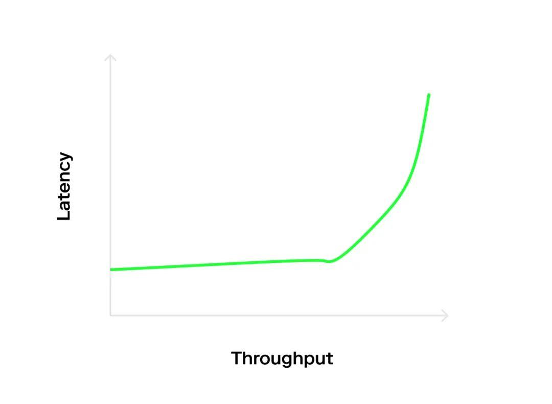
When there is no competition, latency is constant; simply changing the system's load can change throughput. This occurs because, under low competition, the minimum overhead for sending transactions is fixed, and the queue delay is 0, resulting in "whatever comes in can go out directly."

In a highly competitive scenario, throughput is constant, but simply changing the load can cause latency to vary.

This is because the system is already overloaded, and adding more load will cause the waiting queue to grow indefinitely. More strangely, latency seems to change with the length of the experiment, which is an artificial result of an infinitely growing queue.

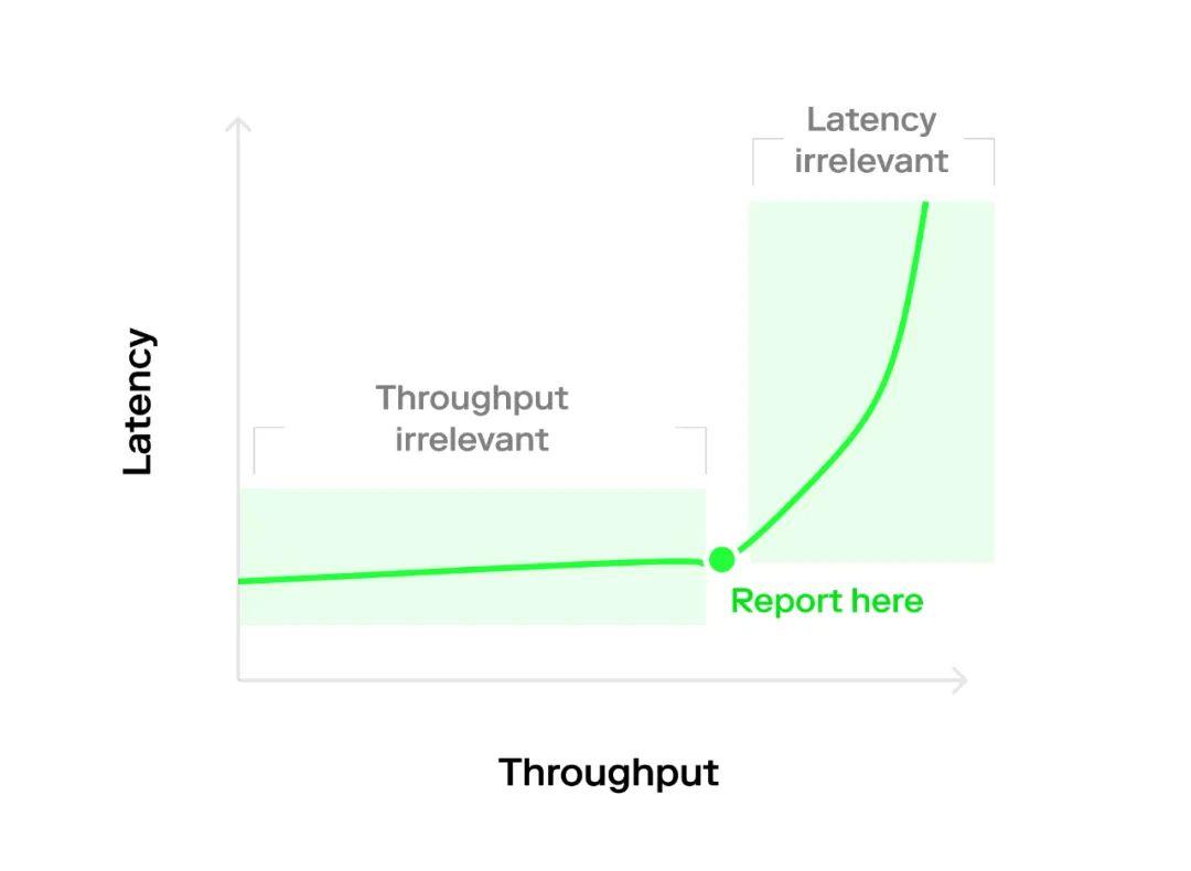
These behaviors can be seen in the typical "hockey stick" or "L-shaped" graphs, depending on the distribution of arrival intervals (which will be discussed below). Therefore, the key point of this article is that we should measure in the hot zone, where both throughput and latency affect our benchmarks, rather than measuring in the edge areas, where only one of throughput or latency is important.

Measurement Methodology

When conducting experiments, the experimenter has three main design options:

1. Open Loop vs. Closed Loop

There are now two main methods to control the request flow to the target. Open-loop systems are modeled based on n = ∞ clients, which send requests to the target based on a rate λ and an arrival interval distribution (e.g., Poisson). Closed-loop systems limit the number of outstanding requests at any given time. The difference between open-loop and closed-loop systems is the characteristics of the specific deployment; the same system can be deployed in different scenarios.

For example, a key-value store can serve thousands of application servers in an open-loop deployment or only a few blocking clients in a closed-loop deployment.

Testing the correct deployment scenario is essential because, compared to closed-loop systems, where latency is often constrained by the potential number of outstanding requests, open-loop systems may generate a large waiting queue, resulting in longer latency. Generally, blockchain protocols can be used by any number of clients, so evaluating them in an open-loop environment will be more accurate.

2. Arrival Interval Distribution for Synthetic Benchmarking

When creating synthetic workloads, we inevitably ask: how do we submit requests to the system? Many systems pre-load transactions before measurement, but this can introduce bias in the measurements because the system starts operating from an anomalous state of 0. Additionally, pre-loaded requests are already in main memory, thus bypassing their network stack.

A better approach is to send requests at a deterministic rate (e.g., 1000 TPS), which will lead to the appearance of an L-shaped graph (orange line) because the system's capacity is optimally utilized.

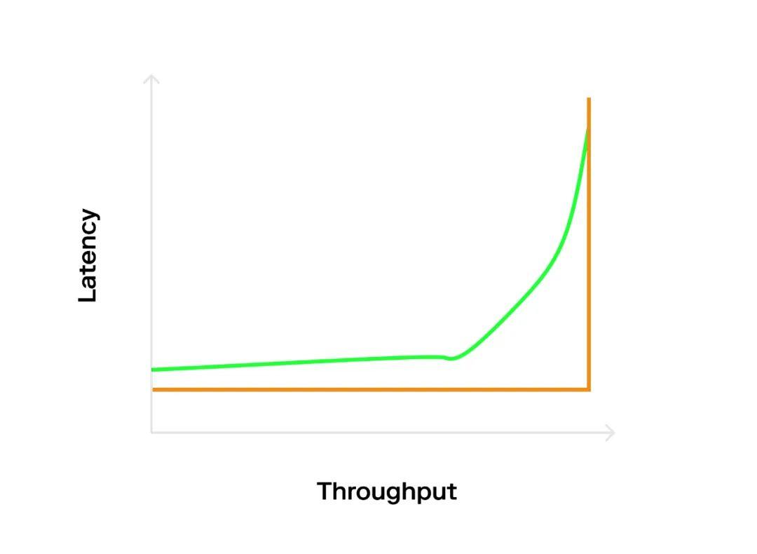
However, open systems often do not operate in a predictable manner. Instead, they have periods of high and low load. To model this, we can use a probabilistic interval distribution, which is generally based on a Poisson distribution. This will lead to a "hockey stick" graph (blue line) because even if the average rate is below the optimal value, Poisson bursts can cause some queuing delays (maximum capacity). But this is very beneficial for us because we can see how the system handles high loads and how quickly the system recovers when the load returns to normal.

3. Warm-up Phase

The last point to consider is when to start measuring. We want the pipeline to be full of transactions before starting; otherwise, we will need to measure warm-up latency. Ideally, the measurement of warm-up latency should be completed through latency measurements during the warm-up phase until the measurement results follow the expected distribution.

How to Compare

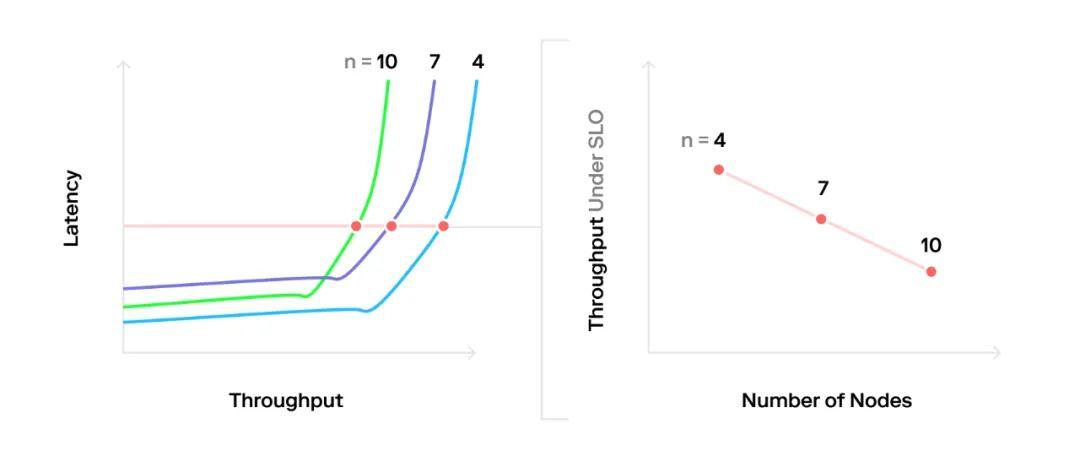
The final challenge is to reasonably compare various deployments of the systems. Similarly, the difficulty lies in the interdependence of latency and throughput, making it difficult to generate a fair throughput/node count graph.

The best approach is to define service level objectives (SLO) and measure the throughput at that time, rather than simply pushing each system to its maximum throughput (in which case latency is meaningless). Plotting a horizontal line on the throughput/latency graph that intersects the SLO on the latency axis and sampling the intersection points is a good visualization method.

But I set a 5-second SLO, and it only takes 2 seconds.

One might want to increase the load here to take advantage of the slightly higher available throughput after the saturation point. However, this is risky. If the system operates underconfigured, an unexpected request burst will cause the system to reach full saturation, resulting in a spike in latency that will quickly violate the SLO. Essentially, operating beyond the saturation point leads to an unstable balance.

Therefore, two points need to be considered:

Overconfigure the system. Essentially, the system should operate below the saturation point to absorb bursts in the arrival interval distribution without causing an increase in queuing latency.

If there is space below the SLO, increase the batch size. This will increase the load on the critical path of the system without increasing queuing latency, providing you with higher throughput for a better latency trade-off.

I am generating huge loads; how should I measure latency?

When the system load is high, trying to access the local clock and adding timestamps for each transaction arriving at the system may lead to biased results.

Instead, there are two more feasible options. The first and simplest method is to sample transactions; for example, there may be a magic number in some transactions, which are the transactions for which the client keeps a timer. After the submission time, anyone can check the blockchain to determine when these transactions were submitted, thus calculating their latency. The main advantage of this approach is that it does not interfere with the arrival interval distribution. However, because certain transactions must be modified, it may be considered "hacky."

A more systematic approach is to use two load generators. The first is the primary load generator, which follows a Poisson distribution. The second request generator is used to measure latency, and its load will be much lower; compared to the rest of the system, this request generator can be viewed as a single client. Even if the system sends replies to each request (as some systems do, such as a key-value store), we can easily place all replies into the load generator and only measure the latency from the request generator.

The only tricky part is that the actual arrival interval distribution is the sum of two random variables; however, the sum of two Poisson distributions is still a Poisson distribution, so the math isn't difficult :).

Conclusion

Measuring large-scale distributed systems is crucial for identifying bottlenecks and analyzing expected behavior under stress. By using the methods outlined above, we hope to take the first step toward a common language, ultimately making blockchain systems more suitable for the work they do and their commitments to end users.

In future work, we plan to apply this method to existing consensus mechanisms, so if you're interested, please reach out on Twitter!